Apache Spark with Python: Building Data Pipelines Step by Step
A hands-on PySpark tutorial covering DataFrame operations, ETL pipeline construction, and Spark 4.0 features. Includes production-ready code examples for data engineers preparing for technical interviews.

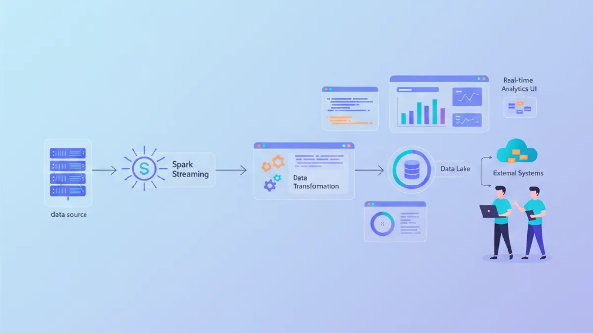
Apache Spark remains the dominant distributed processing engine for large-scale data pipelines in 2026. Combined with PySpark, it offers a Python-native API that handles batch and streaming workloads across clusters of any size without sacrificing performance.
This tutorial walks through building a complete ETL data pipeline with PySpark, from raw ingestion to clean output, using Spark 4.0 features like the Python Data Source API and native DataFrame plotting.
PySpark DataFrames are immutable. Every transformation returns a new DataFrame, leaving the original unchanged. This design enables Spark's lazy evaluation: transformations are only executed when an action (like .show(), .write(), or .collect()) triggers the computation plan.
Setting Up a PySpark 4.0 Environment
Before building any pipeline, the Spark session needs proper configuration. Spark 4.0 enables ANSI mode by default, which enforces stricter SQL semantics — numeric overflows now throw exceptions instead of silently wrapping around.
# spark_setup.py
from pyspark.sql import SparkSession

spark = (
    SparkSession.builder
    .appName("ETLPipeline")
    .config("spark.sql.adaptive.enabled", "true")       # AQE for runtime optimization
    .config("spark.sql.shuffle.partitions", "200")       # Tune based on cluster size
    .config("spark.serializer", "org.apache.spark.serializer.KryoSerializer")
    .getOrCreate()
)

# Verify Spark version
print(spark.version)  # 4.0.0
Adaptive Query Execution (AQE), enabled here, dynamically optimizes shuffle partitions and join strategies at runtime. Spark 4.0 brings 20-50% speedups on typical ETL workloads compared to Spark 3.x, largely through AQE improvements and the Catalyst optimizer.
Reading Raw Data with the DataFrame API
PySpark DataFrames abstract away distributed computation behind a familiar tabular API. Reading from various sources — CSV, Parquet, JSON, databases — follows a consistent pattern.
# read_sources.py
from pyspark.sql.types import StructType, StructField, StringType, DoubleType, TimestampType

# Define schema explicitly — avoids slow schema inference on large files
order_schema = StructType([
    StructField("order_id", StringType(), nullable=False),
    StructField("customer_id", StringType(), nullable=False),
    StructField("product_code", StringType(), nullable=True),
    StructField("amount", DoubleType(), nullable=True),
    StructField("order_date", TimestampType(), nullable=True),
    StructField("region", StringType(), nullable=True),
])

# Read CSV with explicit schema
raw_orders = (
    spark.read
    .schema(order_schema)                    # Skip inference, enforce types
    .option("header", "true")                # First row contains column names
    .option("mode", "DROPMALFORMED")         # Skip rows that don't match schema
    .csv("s3a://data-lake/raw/orders/")
)

# Read Parquet — schema is embedded in the file format
products = spark.read.parquet("s3a://data-lake/raw/products/")

raw_orders.printSchema()
raw_orders.show(5, truncate=False)
Explicit schema definition is a production best practice. Schema inference requires a full scan of the data source, which is expensive on large datasets and can guess types incorrectly (interpreting ZIP codes as integers, for instance).
Cleaning and Transforming DataFrames
Raw data always needs cleaning. PySpark transformations chain naturally using the DataFrame API, and since DataFrames are immutable, each step produces a new DataFrame without modifying the original.
# clean_orders.py
from pyspark.sql import functions as F

cleaned_orders = (
    raw_orders
    .filter(F.col("order_id").isNotNull())                     # Remove null primary keys
    .filter(F.col("amount") > 0)                               # Filter invalid amounts
    .withColumn("customer_id", F.trim(F.upper(F.col("customer_id"))))  # Normalize IDs
    .withColumn("order_date", F.to_date(F.col("order_date")))  # Cast to date type
    .withColumn("year_month",                                   # Extract partition key
        F.date_format(F.col("order_date"), "yyyy-MM"))
    .dropDuplicates(["order_id"])                               # Deduplicate by order ID
)

print(f"Raw: {raw_orders.count()} rows -> Cleaned: {cleaned_orders.count()} rows")
Order matters in transformation chains. Normalizing customer_id before deduplication ensures consistent matching. Extracting year_month after date parsing avoids null values in the partition column.
Calling .collect() pulls the entire distributed DataFrame into the driver's memory. On datasets exceeding the driver's RAM, this causes an OutOfMemoryError. Use .show(), .take(), or .toPandas() on pre-filtered subsets instead.
Joining and Aggregating Across Sources
Real pipelines combine data from multiple sources. PySpark supports all standard join types, and Spark 4.0's AQE automatically selects broadcast joins for small tables without manual hints.
# enrich_orders.py
# Join orders with product catalog
enriched = (
    cleaned_orders
    .join(products, on="product_code", how="left")      # Keep all orders, even unmatched
    .select(
        "order_id",
        "customer_id",
        "product_code",
        F.col("name").alias("product_name"),              # Rename for clarity
        "amount",
        F.col("category"),                                # From products table
        "order_date",
        "year_month",
    )
)

# Aggregate: monthly revenue per product category
monthly_revenue = (
    enriched
    .groupBy("year_month", "category")
    .agg(
        F.sum("amount").alias("total_revenue"),            # Sum all order amounts
        F.countDistinct("order_id").alias("order_count"),  # Unique orders
        F.avg("amount").alias("avg_order_value"),          # Average basket size
    )
    .orderBy(F.desc("total_revenue"))
)

monthly_revenue.show(10)
The left join preserves all orders even when a product code has no match in the catalog — a common scenario during data migration or when product catalogs lag behind transaction systems.
Ready to ace your Data Engineering interviews?
Practice with our interactive simulators, flashcards, and technical tests.
Writing Optimized Output with Partitioning
The final step in an ETL pipeline writes transformed data to a target storage layer. Partitioning the output by frequently-queried columns dramatically reduces read times for downstream consumers.
# write_output.py
# Write enriched data partitioned by year_month
(
    enriched
    .repartition("year_month")                             # Align partitions with output
    .write
    .mode("overwrite")                                     # Replace existing partition data
    .partitionBy("year_month")                             # Physical directory partitioning
    .parquet("s3a://data-lake/curated/enriched_orders/")
)

# Write aggregated metrics as a single compact file
(
    monthly_revenue
    .coalesce(1)                                           # Single output file for small results
    .write
    .mode("overwrite")
    .parquet("s3a://data-lake/curated/monthly_revenue/")
)

print("Pipeline complete — output written to curated layer")
Using .repartition() before .partitionBy() ensures each physical partition contains a reasonable number of files. Without it, Spark may produce hundreds of tiny files per partition — a common anti-pattern known as the "small files problem" that degrades read performance on HDFS and object stores.
Spark 4.0: Python Data Source API for Custom Connectors
Spark 4.0 introduces the Python Data Source API, removing the previous requirement to write custom connectors in Java or Scala. This simplifies integration with proprietary systems, REST APIs, or niche file formats.
# custom_source.py
from pyspark.sql.datasource import DataSource, DataSourceReader
from pyspark.sql.types import StructType, StructField, StringType, IntegerType

class APIDataSource(DataSource):
    """Custom data source reading from an internal REST API."""

    @classmethod
    def name(cls) -> str:
        return "internal_api"                              # Registered source name

    def schema(self) -> StructType:
        return StructType([                                # Define output schema
            StructField("id", IntegerType()),
            StructField("name", StringType()),
            StructField("status", StringType()),
        ])

    def reader(self, schema: StructType) -> "APIDataSourceReader":
        return APIDataSourceReader(self.options)           # Pass options to reader

class APIDataSourceReader(DataSourceReader):
    def __init__(self, options):
        self.endpoint = options.get("endpoint", "")        # API endpoint URL

    def read(self, partition):
        import requests                                    # Import inside read for serialization
        response = requests.get(self.endpoint)
        for record in response.json():
            yield (record["id"], record["name"], record["status"])

# Register and use the custom source
spark.dataSource.register(APIDataSource)
api_df = spark.read.format("internal_api").option("endpoint", "https://api.internal/users").load()
api_df.show()
The Python Data Source API supports both batch and streaming reads. For production use, adding error handling inside read() and implementing partition-level parallelism significantly improves throughput.
Spark Connect decouples client applications from the Spark cluster. The lightweight PySpark client (pyspark-client) weighs only 1.5 MB compared to the full 355 MB PySpark package. This enables running Spark jobs from any IDE or notebook without a local Spark installation.
Performance Tuning Checklist for PySpark Pipelines
Building a pipeline that works is only part of the challenge. Making it performant at scale requires attention to partitioning, caching, and join strategies.
| Technique | When to Apply | Impact |
|-----------|---------------|--------|
| Explicit schemas | Every read operation | Eliminates schema inference scan |
| Partition pruning | Filtering partitioned datasets | Skips irrelevant data partitions entirely |
| Broadcast joins | Small table (< 10 MB) joined to large table | Avoids expensive shuffle |
| Caching | DataFrame reused in multiple actions | Prevents recomputation |
| Coalesce vs Repartition | Reducing partition count | coalesce avoids full shuffle |
| AQE | Always (default in Spark 4.0) | Runtime optimization of joins and shuffles |
Monitoring pipeline performance through the Spark UI remains essential. The DAG visualization reveals shuffle boundaries, and the SQL tab shows the physical plan chosen by the Catalyst optimizer.
Conclusion
- PySpark 4.0 provides a mature, Python-first API for building ETL pipelines at any scale, with ANSI SQL compliance enabled by default
- Explicit schema definition, proper partitioning, and AQE eliminate the most common performance bottlenecks in production pipelines
- The new Python Data Source API removes the Java/Scala barrier for custom connectors — REST APIs, proprietary formats, and streaming sources can all be integrated in pure Python
- Transformation order matters: normalize identifiers before deduplication, parse dates before extracting partition keys
- The Data Engineering interview questions frequently cover Spark internals like lazy evaluation, shuffle mechanics, and partition strategies — understanding these pipeline fundamentals directly prepares for those conversations
- Explore ETL and ELT patterns for deeper coverage of pipeline architecture decisions
Start practicing!
Test your knowledge with our interview simulators and technical tests.
Tags
Share
Related articles
Apache Spark 4 in 2026: New Features, Structured Streaming and Interview Questions
A comprehensive guide to Apache Spark 4.x covering ANSI mode, VARIANT type, Real-Time Mode streaming, Spark Connect, and common data engineering interview questions with code examples.
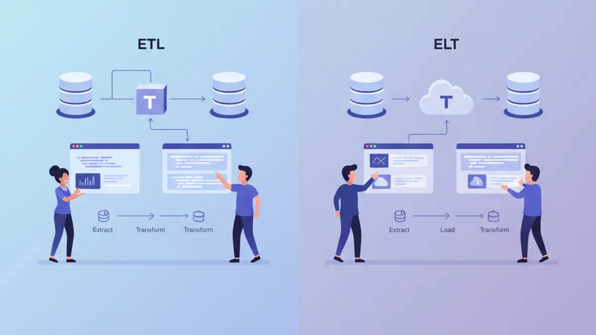
ETL vs ELT in 2026: Data Pipeline Architecture Explained
ETL vs ELT comparison for modern data pipelines. Understand the architectural differences, performance trade-offs, and when to use each approach with Snowflake, BigQuery, and dbt in 2026.
Top 25 Data Engineering Interview Questions in 2026
The 25 most asked data engineering interview questions in 2026, covering SQL, data pipelines, ETL/ELT, Spark, Kafka, data modeling, and system design with detailed answers.